
Representation Geometry Is Not Load-Bearing
Ongoing research. This is an experimental result from active work, not a settled conclusion. The numbers are what we measured and the method is described so you can judge it, but the programme is still running and later experiments may revise what it means.
A note on the language in these records. This is a working laboratory notebook for research into training AI models more cheaply and efficiently, so you will read that an approach did not work, that a result did not hold up, or that one method was worse than another. That is the research doing its job, not a verdict on the engineering we deliver to clients. Ruling an approach out is how the search narrows, and these are the pages that teach us the most: nearly every technique we now rely on came from understanding why something else fell short. Testing our own ideas at least as hard as anyone else's is the point of publishing them. More about this programme and why we run it.
Part of a bigger question: Does reshaping a model's internals make training cheaper? – No. The technique does exactly what it claims and the claim does not translate into an efficiency gain -- ordinary training reaches the same place, and the overhead is 23x the measured benefit.
In plain English
What we asked. When an AI model learns, it spreads information across thousands of internal numbers. We spent a research programme asking whether tidying that spread up, forcing the model to use fewer internal directions, would make training cheaper or better.
What we found. It changes almost nothing. We could strip out 97% of the model's internal spread and lose less than a tenth of a percentage point of accuracy. We tried it on small models and larger ones, on easy problems and hard ones, gently and aggressively. The answer was the same every time.
Why it matters. This is a negative result, and it saved us six months. A lot of published work treats the shape of a model's internals as though it were the thing that matters. On the problems we could test, it is not: the difficulty lives somewhere else. Knowing where not to look is worth as much as knowing where to.
The rest of this page is the technical record: the design, every number, and the limits. It is written for a reviewer, and you do not need it to have understood the result above.
New here? How to read a research record
- Start at the verdict. Every record states, before the experiment was run, what result would have made us abandon the idea. That is the "kill test". Then it says whether the test fired. Nothing gets reinterpreted after the fact.
- Numbers in square brackets are uncertainty.
23.4 [18.1, 28.7]means our best estimate is 23.4 and the true value is probably somewhere in that range. If a range includes zero, we cannot claim an effect. - Results that rule an idea out are kept. Roughly half of what is published here says an approach did not work, including plenty of our own. Those pages are the output, not a shortfall: knowing which direction is a dead end is what lets the next experiment go somewhere better, and most of what we now rely on came out of understanding why something else fell short. Work that only publishes what worked is not measuring anything.
- Read the Limits section. Every record ends with what it does not show. It is the most honest part of any experiment and usually the shortest.
- Pro tip: the figures near the top are designed to carry the result on their own. If you read nothing else, read the caption under each one, which says what it shows and what to take from it.
A small-scale study of low-rank latent structure, its costs, and one confirmed phenomenon
Latent Pretraining Research · Version 0.33.0 · 2026-08-20 Repository: joshuabolick/latent-pretraining-research
Abstract
We set out to test whether encouraging a neural network to concentrate its internal representation into fewer dimensions could make training more efficient. Across 183 archived GPU runs and roughly 600 additional local runs, the answer is no, and the reason turns out to be more interesting than the original question.
We report four results. First, a correction: an effect confirmed across three studies as a distinct "normalisation mechanism" was algebraically identical to the same penalty at a 1.2× larger weight, verified to below float32 epsilon. Second, a priced negative: the compactness the penalty produces is real and reproducible, but ordinary training followed by truncation and a few fine-tuning steps reaches the same place, leaving the intervention roughly 57× underwater; making the penalty 14× cheaper does not change this, because the benefit it buys is not statistically distinguishable from zero. Third, a confirmed phenomenon: latent representations expand by roughly 50% of their baseline residual energy at the learning transition and then consolidate, replicating on unseen seeds against a preregistration, with the geometric peak tracking the accuracy transition at r = 0.983 across a fourfold induced range. Fourth, and most decisive, a null with wide scope: representation geometry can be reshaped almost arbitrarily, 97.3% of the representation's tail eliminated, or 91.2% of the energy the output head most depends on removed, for under one tenth of a percentage point of held-out accuracy, at every model width, task difficulty, target subspace, and penalty weight tested.
The geometry moves reliably during learning. Moving it deliberately changes nothing. It is a correlate of learning, not a lever on it.
Total cloud compute spend across the entire project: $0.78.
1. Introduction
The motivating hypothesis was straightforward. A neural network's hidden state is a vector in some number of dimensions, say 48. If a model could be encouraged during training to place its useful information in a small subspace of that state, the remaining dimensions might be discarded, yielding a smaller and cheaper model at no cost to quality.
This is a plausible idea with a plausible mechanism, and it is cheap to test at small scale. The project built a platform for testing it: immutable experiment definitions, paired multi-seed studies, checksummed result bundles, preregistered decision rules, and a research console. Eight paired studies and 183 runs accumulated over that platform, culminating in a result classified as width transfer supported.
This paper reports what happened when that result was re-examined, and what the re-examination uncovered. Two features of the setting shape everything that follows:
Experiments are effectively free. A full 500-step training run takes about 7.5 seconds on a laptop CPU; a 36-run study costs four minutes and nothing. The binding constraint on this project was never compute: it was which question the rigour was pointed at.
Negative results are the majority of the output. Six hypotheses were screened and five killed. Three claims made during this work were later withdrawn by better evidence from the same work. We regard this as the project functioning correctly, and Section 7 treats the errors as a first-class result.
2. Experimental setup
Models. Two families behind a shared latent-capture interface: a single-layer causal GRU and a single-layer causal transformer, both with a LayerNorm (final_norm) feeding a linear output head. Widths from 12 to 768; most work at width 48 (17,280 parameters).
Tasks. Synthetic sequence tasks with explicit scoring masks. The primary task is synthetic-delayed-copy-v1: a sequence periodic with period lag, where the model must reproduce a token seen lag positions earlier. Difficulty is controlled by lag, vocabulary size, and sequence length.
Evaluation. Three disjoint samples per run: a seeded training stream, a fixed held-out quality batch, and a smaller fixed representation batch. The subspace used for any post-hoc analysis is always fitted on the representation batch and scored on the held-out batch, never on the same data.
The intervention. A differentiable penalty on rank-r residual energy, the fraction of representation variance lying outside the top r principal directions:
`` residual(H, r) = Σ σᵢ² for i ≥ r ÷ Σ σᵢ² for all i total_loss = task_loss + weight · residual(H, r) ``
Minimising it concentrates variance into r directions. Unless stated, r = 8, weight = 0.05, with a 10-step warmup.
Statistics. All comparisons are paired by seed. Intervals are two-sided 95% Student-t. Where multiple arms are compared, Bonferroni correction is applied and stated.
3. The original hypothesis, and a correction
3.1 The claimed mechanism
Three studies (widths 36, 48, 72; 28 matched seed pairs in total) compared two penalty "normalisations": total-energy-fraction, and discarded-dimension-mean, which was reported to improve the retained-rank endpoint by 2.91%, 3.78%, and 4.78% respectively. Every one of the 28 paired comparisons favoured the second, with confidence intervals far from zero. It was classified as a confirmed mechanism and carried forward as the project's preferred method.
3.2 The correction
The two normalisations are related by a constant:
`` total-energy-fraction: penalty = residual discarded-dimension-mean: penalty = residual · W / (W − r) ``
W and r are fixed hyperparameters, so W/(W−r) is a constant. Since the objective is task_loss + weight · penalty, dimension-mean at weight w is exactly total-energy-fraction at weight w · W/(W−r). Not approximately, identically.
Empirical verification at W = 48, r = 8, where the multiplier is 48/40 = 1.2:
| Metric | dimmean @ 0.05 vs fraction @ 0.06 | vs fraction @ 0.05 |
|---|---|---|
final_loss | 0.00e+00 | 1.77e-03 |
final_eval_loss | 6.42e-08 | 1.97e-03 |
final_effective_rank | 2.68e-08 | 3.31e-03 |
final_latent_residual_energy | 3.55e-08 | 4.28e-03 |
Every difference against weight 0.06 is at or below float32 epsilon (1.19e-07). They are the same run.
All three studies fixed retained rank at exactly one sixth of width: 6/36, 8/48, 12/72, holding the multiplier at 1.2 throughout. The project's decision log had already recorded that all three used "the same 1.2 normalization multiplier"; what was not drawn was the implication that holding it constant reduced the treatment arm to a weight change.
The observed effect sizes are what the weight response predicts. Extrapolating the existing GRU weight-response curve to a 1.2× weight increase gives 2.65%, inside the observed 2.91–4.78% range.
3.3 What this cost, and what it teaches
Six releases of confirmatory work measured, three times, that a 20% larger penalty compresses 3–5% more. The 28-of-28 consistency and the tight intervals were not evidence of a mechanism: they are what near-deterministic monotonicity looks like.
Two further limits surfaced in the same review. The primary endpoint, rank-8 residual energy, is the quantity the penalty minimises, making the result close to circular. And held-out accuracy sat at 96–99.5% in every arm, leaving the ±2 percentage point quality guardrail no headroom to detect a trade-off.
4. Pricing the efficiency claim
With the mechanism claim withdrawn, the underlying question remained: does the compactness buy anything?
4.1 Structural reduction
We built the first endpoint in the project that is downstream of the training objective rather than identical to it: project the final representation onto its own top-r subspace and score the output head on the projected states.
On the archived lag=4 task, the penalised model retained 95% of its untruncated accuracy at rank 12 where the baseline needed rank 16, mean 3.2 dimensions saved, 4 of 5 seeds favourable, at an untruncated cost of −0.17 pp. Narrow models trained directly at widths 6–12 reached only 8–33% accuracy, so the reduction was not obtainable by simply building smaller.
On a harder lag=8 task, neither arm reached 95% retention at any rank below full width.
4.2 The cheaper alternative
Post-hoc truncation with no adaptation is the harshest possible test. Allowing a few ordinary fine-tuning steps changes the picture completely: at lag=4, the treatment's 5.2-point rank-8 advantage became a 0.08-point disadvantage, with 5/5 recovery for every arm at every rank.
The apparent surviving advantage was faster recovery, 3.6 steps versus 6.2. Measuring the cost side properly:
| Configuration | 800-step optimiser time | Overhead |
|---|---|---|
Task-only (track_training_residual=false) | 3.60s | , |
| Baseline with metric-only SVD | 4.11s | +14.2% |
| Treatment with penalty | 4.26s | +18.3% |
The penalty's overhead is worth about 147 equivalent training steps, to save about 2.6, roughly 57× underwater.
A measurement trap.trainer.track_training_residualdefaults totrue, so a naive "baseline" computes the same per-step SVD as the treatment purely for metrics. A first attempt at this table compared those two arms and measured the penalty overhead as negative.
4.3 Cost was fixable; benefit was not
The per-step SVD costs O(n·d²) and, measured across widths 48–768, its overhead rises with width (+33.4% to +58.3%), the exponent for the SVD (1.33) exceeds that for the training step (1.08). That closed the case on cost.
Cost turned out to be an engineering problem. A cached-subspace estimator, refreshing the retained basis every k steps and projecting against it in between at O(n·d·r), reverses the trend entirely:
| Width | Exact | Cached (k=50) | Reduction |
|---|---|---|---|
| 48 | +22.3% | +8.9% | 2.5× |
| 192 | +44.8% | +7.7% | 5.8× |
| 768 | +52.2% | +3.7% | 14.1× |
Geometry is preserved: residual energy 0.306013 exact versus 0.305417 cached at width 48.
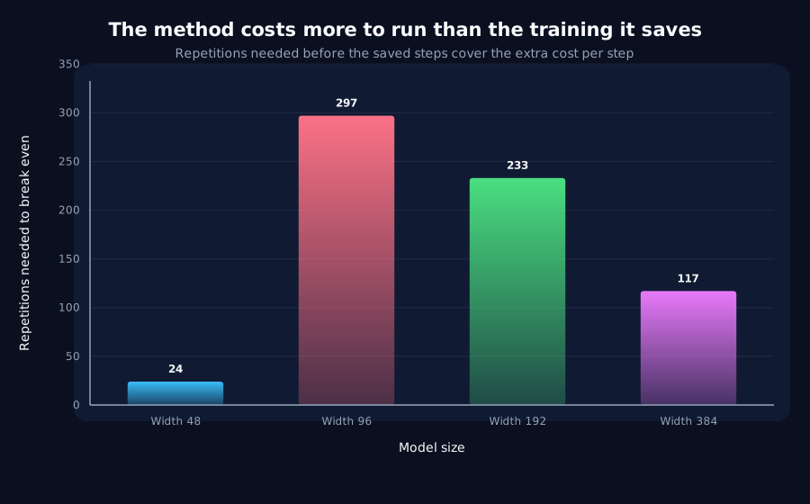
But the benefit does not scale. Measuring both sides per width in the same runs:
| Width | Saved steps | Overhead | Break-even |
|---|---|---|---|
| 48 | 3.0 | +8.9% | 24× |
| 96 | 0.2 | +7.4% | 297× |
| 192 | 0.2 | +5.8% | 233× |
| 384 | 0.4 | +5.9% | 117× |
And critically, no width produces a paired interval excluding zero. Applying the same test to the earlier fine-tuning result gives [−2.18, +7.38]: that benefit was never statistically established either. The direction and the 4-of-5 count were reported accurately; describing it as an effect was not warranted.
5. A confirmed phenomenon: expansion at the learning transition
Every idea screened to this point was a method, and every one lost to a cheaper ordinary alternative. We turned to a question about a phenomenon, which cannot fail that way.
5.1 The observation
Across all 41 archived task-only runs: no penalty, nothing driving geometry but learning itself, rank-8 residual energy rises during training, peaks near the accuracy transition, and then consolidates.
Since residual energy measures variance outside the top 8 directions, a rise means the representation becomes measurably less concentrated while the task is being learned.
5.2 The confounder, and the test that settles it
Every archived run used the same learning rate, so transitions clustered between steps 70 and 120. A peak that merely happened early would look identical; the within-archive correlation was only r = 0.458.
Sweeping learning rate across a 16× range moved the transition from step 55 to 205. The peak followed, at r = 0.954, with the rise positive in 56 of 56 runs.
5.3 Preregistered confirmation
A confirmation was preregistered: design, seeds, endpoints, and decision rules fixed at a commit pushed before any run started, and executed on twelve seeds appearing in no previous study.
| Requirement | Observed | Result |
|---|---|---|
Mean rise ≥ 0.05, interval above zero | +0.2225 [+0.2168, +0.2283] | Pass |
| ≥ 10 of 12 peaks within 50 steps of transition | 12 of 12 (mean offset +2.1) | Pass |
Transition–peak correlation ≥ 0.70 | r = 0.983 | Pass |
| Rise above zero at ranks 4, 8, 16, 24 | all four | not a rank artifact |
| Transformer arm, same rules | +0.0231 [+0.0192, +0.0270] | Fail (materiality floor) |
Preregistered classification: confirmed, architecture-specific. The transformer's interval excludes zero and all twelve runs peak within 50 steps, but at 9.6× weaker magnitude: small, not absent. The threshold was not moved after inspection.
5.4 What sets its size: two withdrawn answers
Magnitude does not track representational difficulty. Across lag 2→8 the rise is flat (+1%) while the transition moves from step 58 to 162, with a constant baseline, a clean null. Across vocabulary 8→64 the rise falls 38%, but the baseline rises tenfold over the same range, making that trend a ceiling artifact.
Normalising by available headroom made both axes flat at 0.305–0.357, and we reported that as a possible invariant. A width sweep withdrew it. Headroom-normalised expansion rises with width under fixed absolute rank (0.253→0.436) and falls under fixed relative rank (0.361→0.260), two opposing trends that cross at exactly width 48, because rank 8 is 48/6 there, and width 48 is where every prior measurement was taken. The invariant was a crossing point.
6. Geometry is not load-bearing
6.1 What the expansion is made of
Decomposing the residual ratio into absolute energies over five seeds, baseline to peak: total energy grows 1.823×, top-8 energy 1.166×, and tail energy 3.150× [3.014, 3.286]. It is genuine expansion into new directions, not redistribution. (Total energy grows because nn.LayerNorm carries a learned affine gain, which roughly doubles over training.)
Meanwhile the output head moves the other way. Its alignment with the representation's top-8 subspace climbs from 0.1905 at initialisation, against a measured chance value of 0.1697, to 0.5745, a 3.4× concentration into one sixth of the space.
This suggested a mechanism: the penalty was free because it suppressed the tail, precisely the part the head learns not to read. That would explain unchanged quality, absent efficiency, and a cross-model CKA of 0.98 all at once.
6.2 The mechanism, falsified by its own test
The mechanism named its own falsification: penalise the head's most-responsive directions and predict a quality collapse. Three penalties, identical in form, differing only in target subspace:
| Arm | Moved its own target by | Accuracy vs control |
|---|---|---|
| tail | −0.2714 (0.4332 → 0.1617) | −0.09 pp [−0.40, +0.21] |
| head-top | −0.2509 (0.4705 → 0.2197) | +0.08 pp [−0.08, +0.25] |
| head-bottom | −0.0390 (0.0950 → 0.0560) | −0.01 pp [−0.18, +0.17] |
Halving the representation's energy in the directions the head responds to most strongly cost nothing. The test was not underpowered, the head penalty moved its target as much as the tail penalty moved its own. The tail penalty pushes energy into head-aligned directions and the head penalty pushes it out; both are free.
6.3 Capacity, also falsified
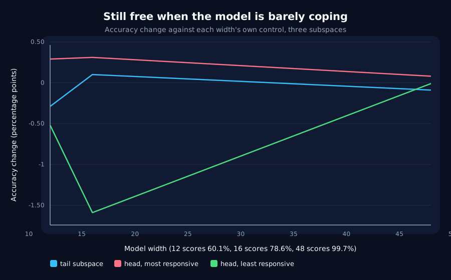
The remaining explanation was that the model simply has more capacity than the task needs. At 30 seeds per arm and widths where the task is genuinely unsolved:
| Width | Control accuracy | tail | head-top | head-bottom |
|---|---|---|---|---|
| 16 | 78.61% | +0.10 | +0.31 | −1.59 |
| 12 | 60.13% | −0.29 | +0.29 | −0.52 |
Nothing binds. The single marginal result (head-bottom at width 16) fails Bonferroni correction ([−3.30, +0.12]), fails to replicate at width 12, and is the wrong arm, penalising what the head reads most was free at both widths.
6.4 The penalty was never too weak
The last untested variable was penalty weight, held at 0.05 throughout for comparability. Sweeping it across two orders of magnitude, reporting achieved geometry alongside accuracy:
| Penalty | Weight | Cost (pp) | 95% interval | Target | Removed |
|---|---|---|---|---|---|
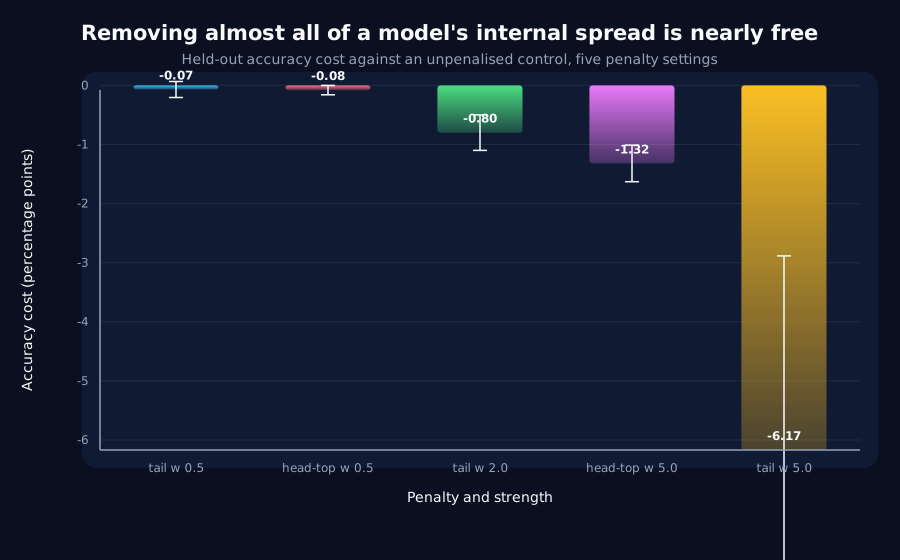
| tail | 0.5 | −0.07 | [−0.20, +0.07] | 0.0115 | 97.3% |
| tail | 2.0 | −0.80 | [−1.10, −0.50] | 0.0151 | 96.5% |
| tail | 5.0 | −6.17 | [−9.45, −2.88] | 0.0116 | 97.3% |
| head-top | 0.5 | −0.08 | [−0.16, −0.00] | 0.0412 | 91.2% |
| head-top | 5.0 | −1.32 | [−1.63, −1.01] | 0.0113 | 97.6% |
At weight 0.5 the tail penalty eliminates 97.3% of the representation's tail, leaving 98.9% of all variance in 8 of 48 directions, for −0.07 pp, an interval including zero.
Beyond weight 0.5 the tail target is flat (0.0115, 0.0151, 0.0116) while cost grows from −0.07 to −6.17 pp. Weight 5.0 costs 88× more accuracy and achieves identical geometry. That is optimisation interference, not a constraint binding, a distinction only visible because achieved geometry was measured alongside accuracy.
6.5 The scope of the null
| Regime | Result |
|---|---|
| Width 48, 99.7% accuracy | free |
| Width 16, 78.6% accuracy | free |
| Width 12, 60.1% accuracy | free |
| Tail subspace | free |
| Head's most-responsive subspace | free |
| Head's least-responsive subspace | free |
Weights 0.05 → 5.0 | free where the constraint is achieved |
The penalty was never too weak, the model was never too large, and the subspace was never the wrong one.
7. What the errors taught
Nine standing diagnostics were adopted, each from a mistake this project actually made. We regard this as the most transferable output of the work.
- Report cross-model CKA against a matched control before any geometry claim. It distinguishes "learned something different" from "same solution, rotated", costs nothing, and would have caught the central error after study one rather than study eight.
- Report a paired confidence interval alongside any favourable-direction count. A 4-of-5 count was twice described as an established effect when its interval was
[−2.18, +7.38]. - Price every claim against the cheapest ordinary alternative. The intervention lost not to a better intervention but to plain fine-tuning, which no study had costed against it.
- The primary endpoint must not be the training objective. Penalising a quantity and reporting it fell is close to circular.
- The task must have quality headroom. At 96–99.5% accuracy the guardrails cannot detect a trade-off.
- Normalise bounded quantities by available headroom before comparing across conditions. The raw endpoint produced a clean, monotone, interval-separated trend in the opposite direction to the truth.
- Never validate an invariant at a single point where two conventions coincide. At width 48 a fixed rank 8 and a fixed
width/6are the same measurement, and two oppositely-sloped curves cross there. - Correct for multiple comparisons and require replication. One of three arms marginally excluded zero at one width; it failed correction and did not replicate.
- Statistical detectability is not the same as mattering. Three consecutive automated verdict rules counted any interval excluding zero as a result. Each was written before its weakness was visible, and each would have produced the wrong headline.
Item 9 deserves emphasis. Automated decision rules encoded before their failure modes are understood will state the opposite of the truth with complete confidence. Every verdict in this paper was checked by hand against the underlying numbers, and three were overridden.
Preregistration is for confirmation, not discovery. The project's early pattern: preregister, run 36 GPU runs, confirm a small effect, spent confirmatory framing on effects nobody had shown to exist. Given that a 36-run study costs four minutes and nothing, the correct order is: screen freely and cheaply, then preregister once an effect is shown to exist. The one preregistration that followed that order (Section 5.3) is the only confirmed positive result in the project.
8. Limitations
This work is small in every dimension that matters for generalisation.
- Two architectures, both single-layer, both tiny. Widths 12–768; most results at width 48 (17,280 parameters).
- One task family: synthetic delayed-copy, plus a simpler arithmetic-sequence task. No natural language, no real data.
- One behavioural measure. Accuracy is argmax-only. Calibration, robustness, and out-of-distribution behaviour could move while accuracy does not, and this is genuinely untested, it is the most plausible way the central null could be wrong.
- One representation site. All penalties and analyses target
final_norm. Weights, embeddings, and the recurrent state itself were not manipulated. - The positive result is architecture-scoped. The expansion is confirmed for a GRU on delayed-copy; the transformer shows it at a tenth the magnitude, below the preregistered materiality floor.
- Sample sizes range from 5 to 30 seeds per arm. Where they are small, we say so, and three results in this paper were withdrawn precisely because a larger or differently-aimed sample contradicted them.
Nothing here should be extrapolated to production-scale models. What can reasonably transfer is the sign of the central result and the methodology in Section 7.
9. Conclusion
We asked whether concentrating a network's latent representation could make training more efficient. It cannot, in this setting, and the reason is more general than the question: the geometry is not carrying the load.
The representation can be crushed into a sixth of its dimensions, or evacuated from the directions the output head most depends on, at a cost of under a tenth of a percentage point: across every width, task difficulty, target subspace, and penalty weight we could reach. The model routes around any constraint of this kind.
Alongside that sits one solid positive: latent representations reliably expand at the moment of learning and then consolidate, confirmed against a preregistration on unseen seeds, with the peak tracking the transition at r = 0.983. Taken together, the two results are sharper than either alone.
The geometry moves reliably during learning. Moving it deliberately changes nothing. It is a correlate of learning, not a lever on it.
Six hypotheses were screened; five were killed. Three claims made during this work were withdrawn by later evidence from the same work. Every correction was appended rather than applied by rewriting history, and every published number re-derives from committed data.
The whole project cost $0.78 in cloud compute.
Where we stop. Every cheap question this setup can answer has been answered. Further arms would generate variations rather than reduce uncertainty. The honest extensions, a second architecture family, a non-synthetic task, behavioural measures beyond argmax accuracy: are different projects, not further runs of this one.
Appendix A: Result index
Every claim traces to a committed study note.
| Release | Result | Note |
|---|---|---|
| v0.15.0 | Normalisation was a reparameterisation | normalization-reparameterization-correction.md |
| v0.16.0 | Structural reduction, first downstream endpoint | structural-reduction-pilot-v1.md |
| v0.17.0 | Fine-tuning substitutes; 57× underwater | truncation-finetune-pilot-v1.md |
| v0.18.0 | Overhead rises with width | overhead-width-scaling-pilot-v1.md |
| v0.20.0 | Cached estimator; 14× cheaper | cheap-subspace-pilot-v1.md |
| v0.21.0 | Benefit does not scale, never significant | benefit-width-scaling-pilot-v1.md |
| v0.22.0 | CKA ≈ 0.98; a change of basis | archive-mining-v1.md |
| v0.23.0 | Gradient-subspace penalty killed (H1) | gradient-subspace-pilot-v1.md |
| v0.24.0 | Quantisation killed (H4) | quantization-pilot-v1.md |
| v0.25.0 | Phase transition survives screening (H6) | phase-transition-pilot-v1.md |
| v0.26.0 | Preregistered confirmation | phase-transition-confirmation-v1-results.md |
| v0.27.0 | Difficulty refuted | difficulty-scaling-pilot-v1.md |
| v0.28.0 | Invariant withdrawn | width-scaling-pilot-v1.md |
| v0.29.0 | Expansion decomposed | expansion-mechanism-pilot-v1.md |
| v0.30.0 | Mechanism falsified | head-subspace-penalty-v1.md |
| v0.31.0 | Capacity falsified | capacity-test-v1.md |
| v0.32.0 | Weight sweep; line closed | weight-sweep-v1.md |
Appendix B: Reproduction
``bash python -m venv .venv python -m pip install -e ".[dev,local-gpu]" python -m pytest && python -m ruff check . && python -m mypy src ``
Every analysis in this paper is a standalone script under analysis/, runnable on a laptop CPU with no GPU and no cost. Archived GPU runs live under results/ with checksummed manifests; binaries use Git LFS.
| Script | Runtime |
|---|---|
archive_mining.py | ~1 min (reads results/ only) |
structural_reduction_pilot.py | ~6 min |
truncation_finetune_pilot.py | ~5 min |
phase_transition.py / _verify.py | ~1 / ~2 min |
phase_transition_confirmation.py | ~8 min |
capacity_test.py | ~50 min |
weight_sweep.py | ~30 min |
Terms on this page
Every piece of vocabulary this record uses, in plain language. Generated from the text above, so it cannot drift out of step with it.
- accuracy
- The fraction of answers a model gets right on questions it was not trained on.
- architecture
- The blueprint of a model: what components it has and how they connect. Two models can be the same size and completely different architectures.
- argmax
- Short for 'the argument that maximises'. A model outputs a score for every possible next token; the argmax is simply whichever one scored highest. Accuracy is measured on the argmax, which is why accuracy is a thresholded quantity: only the winner counts, and by how much it won is discarded.
- baseline
- The thing you compare against. A result without one is not a result.
- calibration
- Working out an instrument's settings from runs whose answer you already know, so it can be used on a run whose answer you do not.
- CKA
- Centred kernel alignment: a score from 0 to 1 for how similar two sets of internal model activity are, where 1 means the same up to rotation and scale.
- confidence interval
- The range in square brackets after a number, as in 23.4 [18.1, 28.7]. It says roughly where the true value probably sits given how much our measurements varied. An interval that includes zero means we cannot rule out no effect at all.
- exponent
- The number in a power law that says how strongly one quantity responds to another. A bigger exponent means a steeper response to the same doubling.
- fine-tuning
- Continuing to train an already-trained model on a new, usually narrower, task.
- gradient
- The direction and amount by which each of a model's internal numbers should change to do slightly better. Training is repeatedly following it.
- GRU
- Gated Recurrent Unit. A compact design for processing sequences one item at a time, with internal switches controlling what it keeps in memory.
- held-out
- Data the model was never trained on, kept back specifically to test it. Scoring a model on data it has already seen measures memorisation, not learning.
- hidden state
- The model's working memory: the internal numbers it carries from one step of a sequence to the next.
- learning rate
- How big a step training takes each time it updates the model. Too small and nothing happens; too big and it never settles.
- multiple comparisons
- The problem that testing many things at once produces convincing looking results by chance. Test twenty-four ideas at a one-in-five error rate and several will look real without being real.
- normalisation
- Dividing a measurement by something else to make it comparable across cases. What you divide by is a choice, and it can change the answer as much as the data does.
- parameters
- The adjustable numbers inside a model. Training is the process of setting them. Model size is usually quoted as a count of these.
- phase transition
- A point in training where a model's performance jumps abruptly from bad to good, rather than improving gradually. Most of this programme is about what happens at that moment.
- post hoc
- Worked out after the fact, rather than decided in advance. We report such checks separately and never let them decide a result, because it is far too easy to find a pattern once you already know the answer.
- preregistration
- Writing down the design, the measurement and the decision rule before running the experiment, and not changing them afterwards.
- quantisation
- Rounding a model's numbers to fewer bits so it takes less memory and runs on smaller hardware, at some cost in accuracy. Spelled quantization in US usage.
- rank
- How many independent directions a set of numbers really uses. A low-rank structure is one that looks high-dimensional but is actually simple underneath.
- recurrent
- A design that reads a sequence one item at a time, carrying memory forward. The main alternative is attention, which looks at everything at once.
- reproducible
- Someone else running the same code on the same inputs gets the same numbers. Every result here is checked this way.
- residual
- How far the data sits from a proposed description of it, after the description has been fitted as well as it can be. A small residual means the description accounts for what was measured; a large one means something is missing.
- residual energy
- Our measure of how much of a model's internal activity is left over after accounting for its few strongest directions. High means the activity is spread out; low means it is concentrated.
- seed
- The number that fixes all the randomness in a training run. Same seed, same run. Running several seeds is how you tell a real effect from a lucky one.
- subspace
- A slice of a model's internal space: some directions kept, the rest ignored.
- SVD
- Singular Value Decomposition. A standard mathematical procedure that breaks a table of numbers into its independent directions, strongest first. It is how we measure internal structure throughout this work.
- transformer
- The architecture behind most modern large language models. It uses attention to look at every part of the input at once, rather than reading in order.
- truncation
- Cutting a record short. Here it means discarding the last part of a finished training run and recomputing a measurement as if the run had stopped earlier, to see whether the answer depends on how long the run went on.
- variance
- How spread out a set of numbers is. Rising variance in a signal means it is becoming more erratic.
- vocabulary
- The set of distinct symbols a model can read and produce.
- width
- How many internal numbers a model uses at each layer. The usual way we vary model size in these experiments.
Get new results as we publish them
Roughly monthly, one finding per email, in plain English first. Including the approaches that turned out not to work, which are usually the useful ones. No sales email.
Double opt-in: we send a confirmation link and add nobody who does not click it. One-click unsubscribe on every email.