How do you know a fine-tuned AI model is actually better?

You measure it. Hold out a portion of the client's real examples so the model never sees them during training, score the plain base model on those held-out questions first, fine-tune, then score again on the identical questions with identical scoring. The difference is the lift. Because the only thing that changed is the fine-tune, the improvement is attributable to it.

Does fine-tuning actually improve accuracy, or is the base model already good enough?

It depends on the task and, critically, on how much data you have. On a public benchmark of 510 lawyer-annotated commercial contracts, a base Qwen3-4B extracted short contract fields at 62.2% accuracy. Fine-tuned on 396 examples it reached 83.5-85.4%, a lift of 21.3 to 23.2 points across three runs. The same model trained on only 48 examples produced a lift inside the noise floor, so the amount of data was the deciding factor rather than the model's ceiling.

How much of our own data do we need to fine-tune a model?

Fewer examples than most people expect, but more than a handful. In our contract-extraction measurements, 48 training examples produced no measurable improvement while roughly 400 produced a 22-point gain. The honest answer for any specific case is that it depends on how varied and how consistent the examples are, which is what a paid readiness assessment measures on the client's own corpus.

Why can't you just use a public AI benchmark score?

Public benchmarks measure general ability on standardised tests, not your work. A model that scores well in the abstract can still be mediocre at reading your contracts or following your policies. Public benchmarks are also increasingly targeted during training, so a high score can reflect test preparation as much as capability. The only benchmark that answers your question is built from your own tasks.

Research record

The Archive as an Instrument

By Joshua Bolick, Awareness Software Group ~19 min read September 2026

Ongoing research. This is an experimental result from active work, not a settled conclusion. The numbers are what we measured and the method is described so you can judge it, but the programme is still running and later experiments may revise what it means.

A note on the language in these records. This is a working laboratory notebook for research into training AI models more cheaply and efficiently, so you will read that an approach did not work, that a result did not hold up, or that one method was worse than another. That is the research doing its job, not a verdict on the engineering we deliver to clients. Ruling an approach out is how the search narrows, and these are the pages that teach us the most: nearly every technique we now rely on came from understanding why something else fell short. Testing our own ideas at least as hard as anyone else's is the point of publishing them. More about this programme and why we run it.

Part of a bigger question: How do we know our own results are real? – Repeatedly, the control rather than the measurement decided the result -- and several striking findings dissolved when the right comparison was finally run.

In plain English

What we asked. We had 183 recorded experiments sitting in a folder. Before running anything new, we asked what could be learned from the ones we already had, for free.

What we found. Two things, and one of them was a warning. A strong-looking relationship between how quickly a model learned and how well it ended up doing turned out to be an illusion: once we compared only models of the same size, it vanished. A second finding, that bigger models learn at predictable moments, held up. We also discovered our archive varied only one setting, not the four we believed it did.

Why it matters. Old data is cheap and tempting, and it is very easy to pull a confident number out of it that means nothing. The pattern here, a correlation that dissolves the moment you control for size, is one of the most common ways honest people mislead themselves.

The rest of this page is the technical record: the design, every number, and the limits. It is written for a reviewer, and you do not need it to have understood the result above.

New here? How to read a research record

Start at the verdict. Every record states, before the experiment was run, what result would have made us abandon the idea. That is the "kill test". Then it says whether the test fired. Nothing gets reinterpreted after the fact.
Numbers in square brackets are uncertainty. 23.4 [18.1, 28.7] means our best estimate is 23.4 and the true value is probably somewhere in that range. If a range includes zero, we cannot claim an effect.
Results that rule an idea out are kept. Roughly half of what is published here says an approach did not work, including plenty of our own. Those pages are the output, not a shortfall: knowing which direction is a dead end is what lets the next experiment go somewhere better, and most of what we now rely on came out of understanding why something else fell short. Work that only publishes what worked is not measuring anything.
Read the Limits section. Every record ends with what it does not show. It is the most honest part of any experiment and usually the shortest.
Pro tip: the figures near the top are designed to carry the result on their own. If you read nothing else, read the caption under each one, which says what it shows and what to take from it.

EXPLORATORY. Not a preregistered study. No new experiments, no training, no GPU, no cost. Reads only the committed results/ bundles.

Program v2 tier 0. Three backlog items in one pass, because they share one loader:

F10, build the meta-analysis harness over the archive.
A9, does when the transition happens predict what the run ends up knowing?
E4: first fit of a transition scaling law, and its variance decomposition.

Decisive computation: analysis/archive_instrument.py over src/latent_pretraining/analysis/archive.py. Output: analysis/archive_instrument.json. Reproduce with python analysis/archive_instrument.py in about ten seconds.

F10: the instrument

latent_pretraining.analysis.archive is now the single loader for committed bundles. It reads experiment.json, run.json, summary.json, metrics.csv, and analysis/representation_trajectory.json into typed records, derives the preregistered transition features once, and emits three tidy tables: per run, per logged step, per capture step and layer. It is standard-library only and does not import torch, so the archive stays readable in an environment that cannot train.

**What a learning transition looks like.** Two things measured at every step of a single training run. The blue line is how often the model gets the answer right on data it has never seen. The orange line is 'residual energy', how much of the model's internal activity lies *outside* the eight directions it uses most. Low residual energy means the model's internal state is compact and concentrated; high means it is spread out. The model sits at chance for about 80 steps, then learns the task in a burst of roughly 40 steps. That burst is what this project calls the transition. Learning here is not gradual. It is a sudden jump, and the model's internal state visibly reorganises at the same moment, the orange line spikes right as the blue line climbs. Everything else in this program is an attempt to work out what that spike is and whether it can be used.

**A strong correlation that turned out to mean nothing.** Each dot is one training run: when it learned the task (left to right) against how accurate it ended up (bottom to top). Looking at all the dots together, there is a strong downward trend, runs that learned later ended up worse. But the colours show why that is misleading: model width drives both. Wider models learn earlier *and* end up more accurate, so the trend across all dots is really just the width effect in disguise. Within any single colour the trend collapses, and the three colours even point in different directions. The apparent finding was an artifact of mixing three different model sizes together. This is why the result was recorded as 'not answerable from the archive' rather than as a discovery.

**When the transition happens is set by model size, not by luck.** Each bar is the average step at which models of a given size suddenly learn the task. The whiskers show how much that varies between runs that differ only in their random starting point. Wider models learn earlier: around step 111 at width 36, step 72 at width 72. The gap between the bars (about 39 steps) is roughly seven times larger than the whiskers (about 5 steps). So the moment of learning is mostly a consequence of how the model was configured, not of chance, which means it can be predicted in advance from the settings alone, to within about ten steps.

**What 183 committed experiments actually cover.** Every experiment this project has run and kept, arranged by which study it belonged to and how wide the model was. Darker cells hold more runs. Blank cells were never run. The archive is deep but narrow. Model width is the only setting that was ever varied: learning rate, task difficulty, and vocabulary size are identical in all 133 runs of the main task. That is why a planned analysis of how timing depends on those settings could only be done for width, and why future sweeps should be saved as full experiments rather than throwaway scripts.

**The internal signal arrives with the transition, never before it.** For every archived run we found two moments: when accuracy jumped, and when the internal 'residual energy' peaked. This counts the gap between them. Bars to the right of zero mean the internal signal peaked *after* the model had already started getting answers right; bars to the left would mean it peaked first. Almost everything sits at or after zero. The internal signal is a companion to learning, not a warning of it. That is the single biggest obstacle in this research program: you cannot use a signal to act *before* an event if the signal only shows up once the event is underway.

This existed to be built because every pilot in analysis/ carried its own bundle walk, its own transition definition, and its own t-critical table. Four of the five discrepancies the 2026-08-22 review found were consequences of that duplication. There is now one definition of each, unit-tested in tests/unit/test_archive.py.

Regression check. Re-deriving the published H6 screen through the harness reproduces it exactly:

Quantity	Harness	Published (H6 pilot)
Runs	41	41
Rise above own baseline	`+0.2131` `[+0.2082, +0.2181]`	`+0.2131` `[+0.2082, +0.2181]`
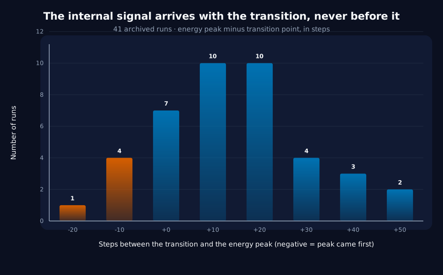
Peak offset from transition	`+14.1` `[+8.9, +19.4]`	`+14.1` `[+8.9, +19.4]`
Peak within 50 steps	100%	100%

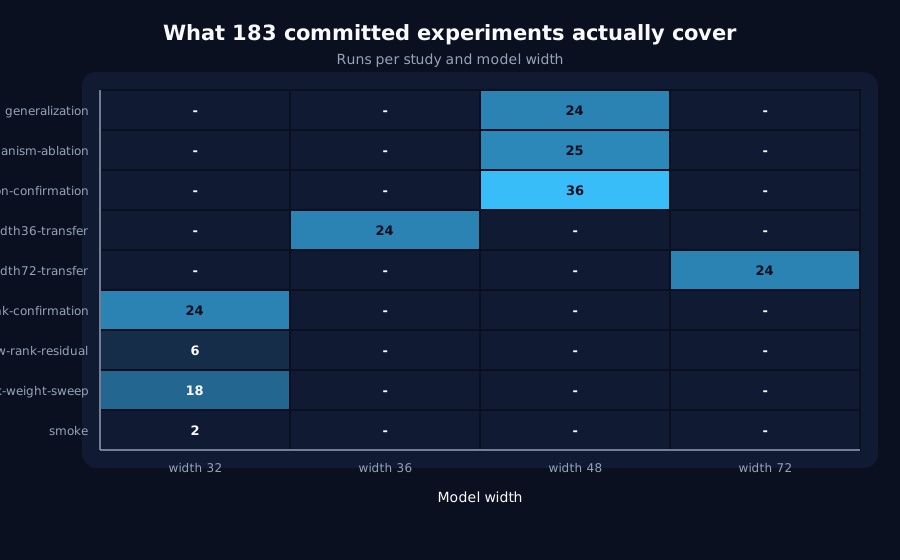
Inventory. 183 bundles: 133 tiny-gru on synthetic-delayed-copy-v1, 50 tiny-transformer on synthetic-v1. 133 logged held-out accuracy, 175 captured a representation trajectory, 57 are task-only, and 41 are task-only and eligible for transition work.

One thing the harness settles immediately, and it is not good news

The backlog's E4 entry assumed "the archive already seeds three of the four axes free". It does not. Across every committed delayed-copy bundle, only three quantities were ever varied: latent width (36 / 48 / 72), penalty weight (0 / 0.025 / 0.05), and retained rank (tied to width at W/6). Learning rate is 0.005, lag is 4, vocabulary is 32, and batch size is 64 in all 133 runs. The lr, lag, and vocabulary sweeps this project has published came from CPU pilots that wrote JSON, not bundles, so their trajectories are not in the archive at all.

That is a standing cost of the pilot convention and it is worth stating plainly: cheap pilots buy answers but do not accumulate an archive. Anything wanting to re-analyse a pilot later must re-run it.

A9: does transition timing matter to the outcome?

Kill test as written: |Spearman rho| < 0.3 between transition step and final held-out accuracy across eligible archived task-only runs.

Verdict: not answerable from the archive. Not a null and not a signal, the measurement does not have the resolution the question needs, in two independent ways.

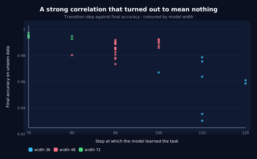
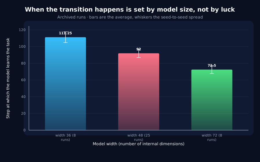
The pooled correlation across all 41 runs is -0.679, which looks decisive and is worthless: width sets both variables. Wider models transition earlier (72.5 steps at width 72, 111.2 at width 36) and finish more accurate. Stratifying by width is mandatory, and it dissolves the result:

Width	Runs	rho	Distinct transition values	Modal tie	Final-accuracy spread
36	8	`-0.316`	3	62%	`0.0485`
48	25	`+0.503`	3	72%	`0.0188` (ceiling-limited)
72	8	`-0.444`	2	75%	`0.0048` (ceiling-limited)

The signs disagree. Only width 48 clears the 0.3 threshold, and it does so in the opposite direction to both other widths. Within width 48 the three contributing studies agree in sign (+0.504, +0.866, +0.308) but each is built on the same two problems:

Timing is quantised to the logging interval. Every archived study logged every 10 steps, so the transition step takes 2–3 distinct values within a width and 72–75% of runs share the modal value. A rank correlation over three tied levels is a two- or three-group mean comparison wearing a correlation's clothes.
The outcome is at the ceiling. Final accuracy spans 0.0048 at width 72 and 0.0188 at width 48. There is almost nothing for timing to rank. This is the saturation problem CLAUDE.md already warns about, showing up in a new place.

Zero of the three strata have both enough timing levels and enough outcome spread to support the test. Reporting -0.679 as an A9 answer would have been this project's third confounded headline.

Second question: does anything at initialisation predict transition time? Pooled, this looks even stronger (initial final_norm effective rank against transition step: rho = -0.776). It is the same width confound: wider models start with higher effective rank and transition earlier. Within width, everything collapses:

Width	Strongest initialisation predictor	rho	n
36	`initial_loss`	`+0.591`	8
48	`init_top_energy_share[embedding]`	`-0.511`	25
72	`initial_loss`	`+0.252`	8

No predictor is consistent across widths, and the two largest come from n = 8 strata where the 5% critical value for Spearman is about 0.71. Consistent with K1: initialisation does not predict transition time either.

What A9 actually needs, and it is cheap: a dedicated pilot at log_every = 1, on a task with real headroom (the E1 battery), across enough seeds to resolve a correlation. That is CPU minutes. A9 moves from "free, archive-only" to "cheap, needs tier 1": it depends on E1.

E4: first fit of a transition scaling law

Kill test as written: across-seed variance at fixed hyperparameters swamps the hyperparameter dependence, making prediction useless at the precision Bucket C needs.

Verdict: survives, on the one axis the archive varies.

Width	Runs	Mean transition step	SD	Range
36	8	111.2	6.4	100–120
48	25	92.0	5.0	80–100
72	8	72.5	4.6	70–80

Width explains eta^2 = 0.853 of transition-step variance.
Between-cell mean spread: 38.8 steps. Within-cell spread: 5.2 steps, falling to 4.4 once the 10-step logging quantisation is removed in quadrature. Ratio 7.4x.
Power law: T ~ width^-0.615, R^2 = 0.859.
Implied scheduling precision: ±10 steps at 95%.

The exponent is the least trustworthy number here, three width points cannot establish a functional form, and the fit is reported for continuity with future sweeps, not as a law. The variance decomposition is the load-bearing part, and it says something the program cares about a great deal.

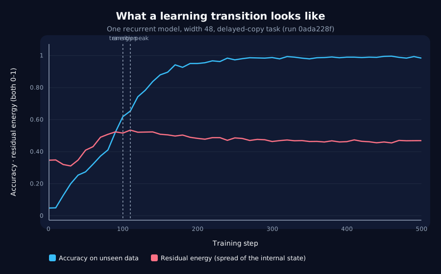
Program v2's central obstacle is that no online signal leads the transition (the geometry peak sits +2.1 steps after it). E4's premise was that this may not matter if timing is predictable from hyperparameters alone, and set the bar at "within a few hundred steps". On the width axis, at fixed everything else, it is predictable to ±10 steps, an order of magnitude better than the bar, on a transition that lands around step 90.

What this does and does not license. It does not deliver a leading indicator: predicting from hyperparameters is an offline schedule, not an online signal, and it is fitted on one axis with three points, at one architecture, on one task, at one learning rate. It does mean the oracle-timing version of A4 (the transition kick) has a non-oracle successor that is not obviously dead, and that a random-time-matched control is testable against a scheduled arm rather than only a retrospective one. The next thing E4 needs is the lr / lag / vocabulary axes measured as committed bundles rather than uncommitted pilots.

What changed in the backlog

Item	Before	After
F10	tier 0, platform	done
A9	tier 0, free, archive-only	archive cannot answer it; needs E1 headroom task + `log_every=1`; moves behind tier 1
E4	tier 3-ish consequence, gated	first fit survives; width dependence is 7.4x seed noise, ±10-step precision; needs the other three axes as bundles
E1	tier 1 platform	now also gates A9

Standing caveat carried forward: everything above is one architecture (tiny-gru), one task (synthetic-delayed-copy-v1), one optimizer (AdamW), one learning rate. D8 (does the phenomenon survive SGD?) and E3 (the architecture × task grid) still scope all of it.

Terms on this page

Every piece of vocabulary this record uses, in plain language. Generated from the text above, so it cannot drift out of step with it.

accuracy: The fraction of answers a model gets right on questions it was not trained on.
AdamW: A widely used training algorithm that adapts how big a step it takes for each individual parameter. The default in most modern AI training.
architecture: The blueprint of a model: what components it has and how they connect. Two models can be the same size and completely different architectures.
baseline: The thing you compare against. A result without one is not a result.
batch size: How many examples the model looks at before updating itself once. Bigger batches give a steadier but more expensive update.
confound: A second explanation you did not control for. If bigger models both learn faster and score higher, then 'fast learners score higher' may be entirely about size and not about speed.
exponent: The number in a power law that says how strongly one quantity responds to another. A bigger exponent means a steeper response to the same doubling.
gated: A design where the model has explicit internal switches deciding what to remember and what to discard at each step. GRUs and LSTMs are gated; plain recurrent networks are not.
GRU: Gated Recurrent Unit. A compact design for processing sequences one item at a time, with internal switches controlling what it keeps in memory.
harness: Everything wrapped around a model when it is used as an agent: its instructions, the tools it can call and how they are named, and how the conversation is laid out.
held-out: Data the model was never trained on, kept back specifically to test it. Scoring a model on data it has already seen measures memorisation, not learning.
kill test: A condition written down before running the experiment that says what result would make us abandon the idea. Fixing it in advance is what stops a disappointing result being reinterpreted as an encouraging one.
learning rate: How big a step training takes each time it updates the model. Too small and nothing happens; too big and it never settles.
optimizer: The algorithm that decides how to change the model given the gradient. AdamW and SGD are two common choices and they behave differently.
power law: A relationship where one quantity changes by a fixed percentage whenever another one doubles, rather than by a fixed amount. Most scaling results in AI are stated this way.
quantisation: Rounding a model's numbers to fewer bits so it takes less memory and runs on smaller hardware, at some cost in accuracy. Spelled quantization in US usage.
rank: How many independent directions a set of numbers really uses. A low-rank structure is one that looks high-dimensional but is actually simple underneath.
seed: The number that fixes all the randomness in a training run. Same seed, same run. Running several seeds is how you tell a real effect from a lucky one.
SGD: Stochastic Gradient Descent. The simplest training algorithm: take a step in the direction the gradient points, every time, with no adaptation.
transformer: The architecture behind most modern large language models. It uses attention to look at every part of the input at once, rather than reading in order.
variance: How spread out a set of numbers is. Rising variance in a signal means it is becoming more erratic.
vocabulary: The set of distinct symbols a model can read and produce.
width: How many internal numbers a model uses at each layer. The usual way we vary model size in these experiments.

The plain-language version. This page is the record: the design, the numbers and the limits. If you would rather have the story, The Archive as an Instrument, explained without the jargon, covers the same result for a reader who has never seen a training curve.

About this record. This page is the write-up of an experiment we ran ourselves. Every number on it comes from a run we recorded, and the script that produced each one is named in the text above. We publish these results and the data behind them here, including the ones that went against what we expected.