
Eight Runs Is Not Enough
Ongoing research. This is an experimental result from active work, not a settled conclusion. The numbers are what we measured and the method is described so you can judge it, but the programme is still running and later experiments may revise what it means.
A note on the language in these records. This is a working laboratory notebook for research into training AI models more cheaply and efficiently, so you will read that an approach did not work, that a result did not hold up, or that one method was worse than another. That is the research doing its job, not a verdict on the engineering we deliver to clients. Ruling an approach out is how the search narrows, and these are the pages that teach us the most: nearly every technique we now rely on came from understanding why something else fell short. Testing our own ideas at least as hard as anyone else's is the point of publishing them. More about this programme and why we run it.
Part of a bigger question: How do we know our own results are real? – Repeatedly, the control rather than the measurement decided the result -- and several striking findings dissolved when the right comparison was finally run.
In plain English
What we asked. Two of our earlier experiments happened to use identical settings and the same eight starting points. Because a training run is exactly repeatable given its starting point, those two experiments had unknowingly measured the very same runs from different angles. So we could ask a brand new question by simply joining the two sets of results together, at no cost and with no new computation. The question: does the size of a model's internal adjustments predict how much damage is done by removing part of them?
What we found. Eight runs cannot answer it. Two of our comparisons passed the standard statistical test, but they pointed in opposite directions, which cannot both be true: the same thing cannot make removing the important part more damaging while making removing a random part less damaging. And when we asked what range of values the data was genuinely consistent with, every answer included zero, meaning no relationship at all.
Why it matters. We are publishing this because of what our first analysis did. It used only the standard test, ignored the range, and confidently announced a discovery: that one simple measurement links two things we had never been able to connect. That would have been a notable result. It was eight data points in a lucky arrangement. The uncomfortable part is that we had written a whole earlier report about this exact mistake, three write-ups previously, and then made it anyway. The check that catches it costs nothing and now runs automatically: require the test and the range to agree, and be suspicious when two related comparisons disagree about which direction the effect goes. We have since run the missing experiment. Doing it properly meant repeating the more expensive of the two original experiments on three times as many runs, which is the only thing that could widen the join. The answer came back yes: the size of a model's internal adjustments really does predict how costly it is to remove the part that carries the learning, and now only that one comparison survives while the control correctly shows nothing. We also checked the obvious objection, that both numbers might just reflect how quickly a particular run happens to learn, and it is not that. So the original announcement turned out to be pointing at something real. It was still right to withdraw it, because at the time we had no way of knowing, and a claim that happens to be true for bad reasons is not a result.
The rest of this page is the technical record: the design, every number, and the limits. It is written for a reviewer, and you do not need it to have understood the result above.
New here? How to read a research record
- Start at the verdict. Every record states, before the experiment was run, what result would have made us abandon the idea. That is the "kill test". Then it says whether the test fired. Nothing gets reinterpreted after the fact.
- Numbers in square brackets are uncertainty.
23.4 [18.1, 28.7]means our best estimate is 23.4 and the true value is probably somewhere in that range. If a range includes zero, we cannot claim an effect. - Results that rule an idea out are kept. Roughly half of what is published here says an approach did not work, including plenty of our own. Those pages are the output, not a shortfall: knowing which direction is a dead end is what lets the next experiment go somewhere better, and most of what we now rely on came out of understanding why something else fell short. Work that only publishes what worked is not measuring anything.
- Read the Limits section. Every record ends with what it does not show. It is the most honest part of any experiment and usually the shortest.
- Pro tip: the figures near the top are designed to carry the result on their own. If you read nothing else, read the caption under each one, which says what it shows and what to take from it.
EXPLORATORY. Not a preregistered study. Archive-only, no training at all, no GPU, no cost.
Program v2 Bucket J, item J6. Decisive computation: analysis/magnitude_concentration.pyanalysis/magnitude_concentration.jsonpython analysis/magnitude_concentration.py.
The question
I3 swept five cheap covariates against the leading gradient direction's mass on the recurrent diagonal, and exactly one survived a family-wise null: the gradient buffer's norm at the transition, r = -0.576 against a critical 0.505. Smaller gradients, more of the leading direction on the diagonal.
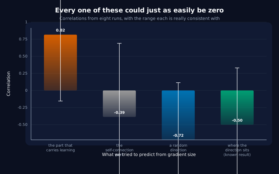
That hints gradient magnitude governs update concentration. J6 asks whether the same variable predicts something that matters, the cost J3's surgery imposes.
It cost nothing to ask. I3 and J3 used the same width, task, learning rate, step count, window and buffer, and the same eight seeds. A run is deterministic given its seed, so I3's buffer norm and J3's surgery cost are measurements of the same trajectory. The whole experiment is a join on the seed, and the script asserts the configurations match before doing it.
Kill test: buffer norm predicts neither the surgery cost nor the lead beyond a family-wise null.
Result: not answerable at this sample size
| Outcome | r | 95% interval | p |
|---|---|---|---|
| off-diagonal surgery cost | +0.816 | [-0.155, +0.986] | 0.025 |
| diagonal surgery cost | -0.387 | [-0.897, +0.689] | 0.340 |
| span-random surgery cost | -0.722 | [-0.966, +0.114] | 0.031 |
| I3's anchor (diagonal mass) | -0.501 | [-0.926, +0.330] | (anchor) |
Two arms clear p < 0.05. Every interval spans zero. And the two significant ones have opposite signs.
That last point is what settles it. The same variable cannot sensibly make removing the load-bearing off-diagonal component more costly while making removing a random direction less costly. Those two arms differ only in which directions were taken out. A predictor that pushes them in opposite directions is not describing a mechanism; it is describing eight points.
The join is sound. I3's own correlation reappears on this subset at r = -0.501 against -0.576 on its full 24 seeds, so the two pilots really are measuring the same trajectories and the sample is the problem, not the plumbing.
What this record is really about
The verdict logic keyed on p < 0.05 alone at first, and reported the kill test as failing. It printed a confident claim that gradient magnitude links composition to consequence, which would have been this programme's first single variable to do so.
That is precisely the failure J1 was written about, committed inside Bucket J, three records after J1. A permutation p and a bootstrap interval disagree constantly at n = 8: a correlation can clear p < 0.05 while its interval spans almost the entire range from -1 to +1. That is not a finding, it is a small sample with a lucky arrangement.
The script now requires both to agree before calling anything resolved, and adds a coherence check on the signs. Both are cheap, and either alone would have caught this.
Verdict
- Not answerable at
n = 8. No claim is made about whether gradient magnitude governs the surgery cost. - I3's original finding is undisturbed and is reproduced here as an anchor.
- The one expensive thing Bucket J has asked for. Resolving this needs J3's surgery re-run at 24 seeds: four arms, so roughly 96 runs and about two hours on a throttled CPU. That is the only item in this bucket that is not effectively free, and it should be weighed against J7 and J8, which are cheaper and ask larger questions.
Limits
- Eight seeds, one width, one task, one learning rate, one window position. Everything above is a statement about sample size, not about the world.
- Bootstrapping a correlation at
n = 8is itself unreliable, and the intervals should be read as "very wide" rather than as calibrated. They are reported because the point estimates alone would be worse. - The join relies on determinism given a seed. That holds here (same code path, same configuration, CPU-only), and the script checks the configuration keys, but it is an assumption worth naming.
- A null from an underpowered test is not evidence of absence. If the effect is real and of the size the point estimates suggest, 24 seeds would resolve it comfortably.
Resolved at 24 seeds, 2026-08-25: the kill test fails, and the confound does not explain it
This section is appended. Nothing above it has been changed, including the "not answerable" verdict, which was correct for the sample it had. Decisive computation is the same committed script, now with the control described below; output analysis/magnitude_concentration.json
The record above named exactly what would resolve this: J3's surgery re-run on I3's 24 seeds. That has now been done, and it was worth doing twice over, because it also re-tested J3's own headline.
J3 reproduces at three times the sample
| Arm | 8 seeds | 24 seeds |
|---|---|---|
| diagonal | +5.3 [+4.4, +6.2] | +5.6 [+5.0, +6.2] |
| off-diagonal | +34.5 [+32.7, +36.3] | +34.5 [+33.8, +35.2] |
| span-random | +3.6 [+2.8, +4.4] | +3.5 [+3.2, +3.8] |
| paired, diagonal − off-diagonal | -29.2 [-31.7, -26.6] | -28.9 [-30.0, -27.9] |
Resolved 24/24, energy matched to 1.2% across arms. J1 and J2 said to re-run the headlines that were found by looking; J3's was one, and it holds with intervals roughly 2.4x tighter.
J6 now resolves, and only one arm does
| Outcome | r | 95% interval | p | partial r | partial p |
|---|---|---|---|---|---|
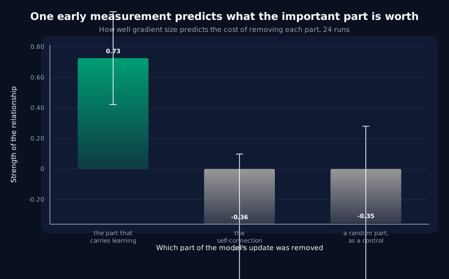
| off-diagonal surgery cost | +0.726 | [+0.422, +0.893] | 0.0001 | +0.708 | 0.0004 |
| diagonal surgery cost | -0.362 | [-0.632, +0.097] | 0.0863 | -0.439 | 0.0391 |
| span-random surgery cost | -0.355 | [-0.695, +0.280] | 0.0887 | -0.401 | 0.0568 |
| I3's anchor (diagonal mass) | -0.576 | [-0.816, -0.369] | (anchor) |
The incoherence is gone. At n = 8 two arms cleared p < 0.05 with opposite signs, which is what forced the original verdict. At n = 24 exactly one arm resolves, the other two fall below p < 0.05 and keep intervals spanning zero, and the surviving one is the arm J3 showed actually carries the learning.
Note the diagonal arm's partial p of 0.0391: it clears p < 0.05 while its bootstrap interval still spans zero, so the rule this record was written about correctly refuses it. The check that caught the original error is still doing work.
The control a positive result needs
Both the predictor and the outcome could simply track how fast a seed happens to learn. A run that transitions later has had longer for its gradients to shrink and a different amount of training behind the window the surgery acts in. That would produce this correlation with no mechanism at all.
So the script now computes the partial correlation holding each seed's own transition step fixed, with its own permutation null, and requires a result to survive it before reporting it.
It survives: +0.708 against a raw +0.726. The confound explains almost none of it, and both of its legs are weak, buffer norm against transition step is +0.241, transition step against cost is +0.391.
The chain is internally coherent
The two numbers point opposite ways, and that is what makes them believable together:
- **Bigger gradient norm → less diagonal mass** in the leading direction (I3's anchor,
-0.576). - Less diagonal mass → more of the direction lies off-diagonal, which is the component J3 showed carries the learning at
6.5xthe diagonal's cost at matched energy. - So bigger gradient norm → removing the off-diagonal component costs more (
+0.726).
The anchor and the outcome have opposite signs, which is exactly what that chain predicts and not what a shared-cause artifact would produce.
Verdict
- The kill test fails. Gradient magnitude at the transition predicts both how concentrated the update is and what removing part of it costs. This is the first single variable in the programme to link composition to consequence.
- It survives the obvious confound, which is the only reason it is being reported as a finding rather than as an association.
- The original "not answerable" verdict was right for its sample, and the sample was the problem, exactly as this record predicted.
Limits on the resolved result
- This is a correlation across seeds, not an intervention. Nothing here manipulates the gradient norm and watches the cost follow. That experiment is not in the backlog yet and would be the natural successor.
- 24 seeds, one width, one task, one learning rate, one window position. J5 is the standing warning: a width-48 fact in this programme has already turned out once to be a fact about width 48 rather than about the phenomenon.
- The predictor was found by looking. I3 paid a family-wise price to select buffer norm from five covariates; this tests it against a new outcome, which is a single prespecified test, but the variable itself still arrived by search.
- The partial correlation controls for one confound, the one with an obvious mechanism. It is not a full causal adjustment.
Terms on this page
Every piece of vocabulary this record uses, in plain language. Generated from the text above, so it cannot drift out of step with it.
- bootstrap
- A way of estimating how uncertain a number is by repeatedly resampling the data you already have. Useful when the usual formulas do not apply.
- calibrated
- A model is calibrated when its confidence matches how often it is right: answers it gives with 90% confidence should be right about 90% of the time.
- confound
- A second explanation you did not control for. If bigger models both learn faster and score higher, then 'fast learners score higher' may be entirely about size and not about speed.
- gradient
- The direction and amount by which each of a model's internal numbers should change to do slightly better. Training is repeatedly following it.
- kill test
- A condition written down before running the experiment that says what result would make us abandon the idea. Fixing it in advance is what stops a disappointing result being reinterpreted as an encouraging one.
- learning rate
- How big a step training takes each time it updates the model. Too small and nothing happens; too big and it never settles.
- recurrent
- A design that reads a sequence one item at a time, carrying memory forward. The main alternative is attention, which looks at everything at once.
- seed
- The number that fixes all the randomness in a training run. Same seed, same run. Running several seeds is how you tell a real effect from a lucky one.
- width
- How many internal numbers a model uses at each layer. The usual way we vary model size in these experiments.
Get new results as we publish them
Roughly monthly, one finding per email, in plain English first. Including the approaches that turned out not to work, which are usually the useful ones. No sales email.
Double opt-in: we send a confirmation link and add nobody who does not click it. One-click unsubscribe on every email.